Lab 5: Sampling
Signals exist in continuous time but it is not unusual for us to process them in discrete time. When we work in discrete time we say that we are doing discrete signal processing, something that is convenient due to the relative ease and lower cost of using computers to manipulate signals. When we use discrete time representations of continuous time signals we need to implement processes to move back and forth between continuous and discrete time. The process of obtaining a discrete time signal from a continuous time signal is called sampling. The process of recovering a continuous time signal from its discrete time samples is called signal reconstruction or interpolation.
• Click here to download the assignment.
Sampling without aliasing
In the first problem of the lab $\textbf{(1.1)}$, you are asked to answer why sampling entails no loss of information for bandlimited signals with bandwith $W$; you are also asked to explain how the signal $x(t)$ can be recovered from the sampled signal $x_s(t)$.
For any sampling frequency $f_s \geq W$, since $X(f) = 0$ for all $f \notin [-W/2,W/2]$, $X[f-kf_s] = 0$ for all $f \notin [kf_s-f_s/2,kf_s+f_s/2]$. This implies $X[f-kf_s]$ and $X[f-lf_s]$ will not overlap for any $k \neq l$. For this reason, upon sampling the spectrum $\sum_{k=-\infty}^\infty X[f-kf_s]$ is periodized but not aliased and sampling entails no loss of information.
In order to recover $x(t)$ perfectly, we low pass filter the the Dirac train representation $x_\delta(t)$ with frequency threshold $\pm f_s/2$, that is,
\begin{equation}
\tilde{x} = x_\delta * [f_s \mbox{sinc}(\pi f_s t)]\ .
\end{equation}
When signals are not bandlimited, loss of information is inevitable. Indeed, when non-bandlimited signals are sampled the spectral content in frequencies above $f_s/2$ and below $-f_s/2$ becomes aliased as exemplified by the red curve in Figure 1. In problem $\textbf{(1.2)}$, you are asked to explain how it is possible to avoid aliasing through judicious use of a low-pass filter.

To avoid distortion we preprocess $x$ with a low pass filter, i.e., we transform $x$ into a signal $x_{f_s}$ with spectrum $X_{f_s} = \ccalF(x_{f_s})$ where $X_{f_s}(f) = X(f)\sqcap_{f_s}(f)$. This can be implemented as a convolution in the time domain,
\begin{equation}
x_{f_s} = x * f_s \mbox{sinc}(\pi f_s t)\ .
\end{equation}
The signal $x_{f_s}$ has bandwith $f_s$ and can be sampled without aliasing. In other words, frequency components between $-f_s/2$ and $f_s/2$ are retained without distortion.
Reconstruction with arbitrary pulse trains
While it is mathematically possible to reconstruct $x(t)$ from $x_\delta(t)$, it is physically implausible to generate a Dirac train. However, we can approximate $\delta(t)$ with narrow pulses $p(t)$. In problem $\textbf{(1.3)}$, you are asked to derive the conditions on $p(t)$ that minimize signal distortion.
To start, the spectra of the actual modulated train pulse using $\delta(t)$ and the approximated modulated train pulse using $p(t)$ can be denoted
\begin{align}
X_\delta(f) &= \sum_{k=-\infty}^{\infty} X(f-kf_s), \\
X_p(f) &= P(f)X_\delta(f) = P(f)\sum_{k=-\infty}^{\infty}X(f-kf_s),
\end{align}
where $P(f)$ is the spectrum of $p(t)$. The reconstruction method described in $\textbf{(1.1)}$ recovers the signal by low pass filtering the sampled signal in the frequency domain. Using this approach, the spectrum $\tilde{X}_\delta (f)$ of the reconstructed signal using $X_\delta(f)$ and the spectrum $\tilde{X}_p(f)$ of the reconstructed signal using $X_p(f)$ can be computed as
\begin{align}
\tilde{X}_\delta(f) &= \sqcap_{f_s}(f)\sum_{k=-\infty}^{\infty} X(f-kf_s) = \sqcap_{f_s}(f)X(f), \\
\tilde{X}_p(f) &= \sqcap_{f_s}(f)P(f)\sum_{k=-\infty}^{\infty} X(f-kf_s) = P(f)\sqcap_{f_s}(f)X(f),
\end{align}
where we use the fact that the low pass filter eliminates all frequencies outside of $[-f_s/2,f_s/2]$. Notice that $\tilde{X}_\delta(f)$ coincides with $\tilde{X}_p(f)$, i.e., no distortion results from using $p(t)$ to approximate $\delta(t)$, when the spectrum of $p(t)$ satisfies
\begin{equation}
P(f) = 1,\mbox{ for all } f \in [-f_s/2,f_s/2].
\end{equation}
In particular, a pulse satisfying this property is $p(t) = f_s\mbox{sinc}(\pi f_s t)$ with $P(f) = \sqcap_{f_s}(f)$. Interestingly, this pulse is not that narrow.
Subsampling
In problem $\textbf{(2.1)}$, you are asked to derive a theorem relating the spectrum of the discrete time signal $x$ and its subsampled version $x_\delta$. Starting from equation (11) of the handout, note that it is equivalent to write
\begin{equation}
x_\delta(n) = x(n) \sum_{m=-\infty}^{\infty} \delta\left(n – m \frac{\tau}{T_s}\right)
\end{equation}
which is $x(n)$ multiplied with a train of discrete deltas with spacing time $\tau$ and sampling time $T_s$. Suppose the sampling time is $\tau$; the train of discrete deltas becomes $\sum_{m=-\infty}^{\infty} \delta(n-m)$ which is a discrete time constant, and its DTFT is a Dirac train with spacing $\nu = 1/\tau$ (see slides 30-32 in the sampling lecture). The following equation in the DTFT derivation will be used later,
\begin{equation}
\tau \sum_{n=-\infty}^{\infty} e^{-j2\pi f n \tau} = \sum_{k=-\infty}^{\infty} \delta(f-k\nu)\ .
\end{equation}
Back to our setting where the sampling time is $T_s$, the train of discrete deltas is a discrete signal with values either $0$ or $1$, depending on whether $n$ is a multiple of $\tau/T_s$. Its DTFT can be computed as
\begin{equation}
X_c(f) = T_s \sum_{n=-\infty}^{\infty} \sum_{m=-\infty}^{\infty} \delta(n – m\tau/T_s) e^{-j 2 \pi f n T_s}\ .
\end{equation}
We may define $n’ = n T_s/\tau$ and utilize the result from (9) in evaluating (10),
\begin{align}
X_c(f) = T_s \sum_{n’=-\infty}^{\infty} \sum_{m=-\infty}^{\infty} \delta(n’ – m) e^{-j2 \pi f n’ \tau} &= T_s \sum_{n’=-\infty}^{\infty} e^{-j2 \pi f n’ \tau} \\
&= \frac{T_s}{\tau} \sum_{k=-\infty}^{\infty} \delta(f-k\nu)\ .
\end{align}
The multiplication in the time domain in (8) implies that the spectrum $X_\delta(f)$ of $x_\delta(n)$ can be written as the convolution of $X(f)$ and the spectrum of the train of discrete deltas. Therefore, we may write
\begin{equation}
X_\delta(f) = X(f) * \frac{T_s}{\tau} \sum_{k=-\infty}^{\infty} \delta(f-k\nu) = \frac{T_s}{\tau} \sum_{k=0}^{\tau/T_s – 1} X\left(f-\frac{k}{\tau}\right)\ .
\end{equation}
In the above derivation, we encountered two entities that appear to be similar — the train of discrete deltas $\sum_{m=-\infty}^{\infty} \delta(n – m \tau/T_s)$ and the Dirac train $\sum_{k=-\infty}^{\infty} \delta(f – k \nu)$ — and here we emphasize their difference. The train of discrete deltas $x(n) = \sum_{m=-\infty}^{\infty} \delta(n – m \tau/T_s)$ is a discrete signal and $x(n)=1$ whenever $n$ is a multiple of $\tau/T_s$ and zero otherwise. The Dirac train $\sum_{k=-\infty}^{\infty} \delta(f – k \nu)$, on the other hand, is a continuous signal and for each $k \in \mbZ$ there is a Dirac delta function (which is a continuous signal itself) centered at $k \nu$. When $\tau = T_s$, $x(n) = \sum_{m=-\infty}^{\infty} \delta(n – m \tau/T_s) = \sum_{m=-\infty}^{\infty} \delta(n-m)$ is also called a discrete time constant.
This spectrum periodization result is verified in problems $\textbf{(2.2)}$ and $\textbf{(2.3)}$. The gaussian pulse sampled at $f_s = 40$kHz with duration $T=2$ and parameters $\mu=1$ and $\sigma=0.1$ is shown on the top of Figure 2. Its subsampled version, with subsampling frequency $\nu = 4$kHz, is shown on the bottom of the same figure.
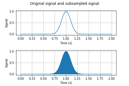
There is not much of a difference between these two signals in the time domain, but if we looks at their DFTs as shown in Figure 3, we see that the DFT of $x_\delta$ is equal to the DFT of $x$ modulated by a Dirac train with spacing $\nu$.
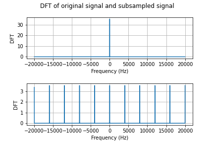
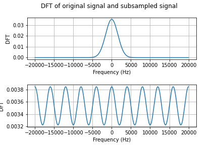
Because the DFT of $x$ is so narrow, there is no aliasing in Figure 3. But if we decrease $\sigma$ to $10^{-4}$, the DFT of the pulse becomes wider and we can see aliasing of consecutive periods of the DFT of $x_\delta$ as in Figure 4.
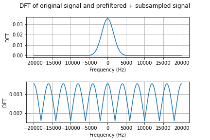
To avoid aliasing, in problems $\textbf{(2.4)}$ and $\textbf{(2.5)}$ we add a prefiltering step before subsampling. The DFT of the gaussian pulse with $\sigma=10^{-4}$, prefiltered to eliminate frequency components outside of the range $[-f_s/2,f_s/2]$, and subsequently subsampled with $\nu=4$kHz, is shown in Figure 5.
Reconstruction
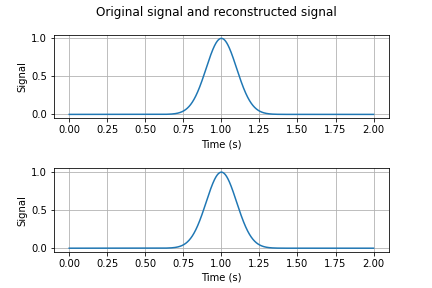
In problem $\textbf{(2.6)}$, you are asked to reconstruct the pulses you subsampled. We start by reconstructing the subsampled gaussian pulse with $\sigma=0.1$. The original and the reconstructed signal are shown in Figure 6. Notice that for this pulse subsampling is lossless as the original signal and its reconstruction have the same shape and energy.
Next, we reconstruct the pulse with $\sigma=10^{-4}$ that was subsampled without prefiltering. The original and reconstructed signals are shown in Figure 7.
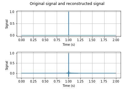
Notice that while the reconstructed pulse seems to have the same energy as the original pulse, it is not a faithful reconstruction because of aliasing. If we now reconstruct the subsampled version of this pulse that was previously prefiltered to avoid aliasing, the reconstructed signal is as in Figure 8.
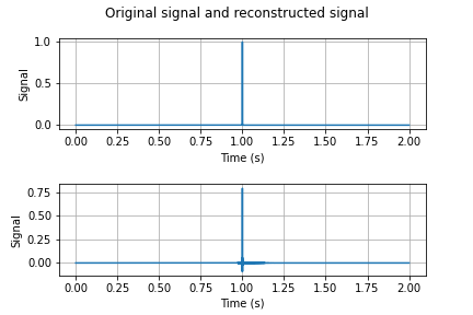
The reconstructed signal clearly has less energy than the original signal, but because there was no aliasing its shape is slightly more faithful to the shape of the original gaussian pulse.
Code links
The classes provided for Lab 5 can be found in the following folder: ESE224_Lab5_provided.zip. This folder contains the following 3 files:
- $\p{dft.py}$: The class $\p{dft}$ implements the discrete Fourier transform in $3$ different ways.
- $\p{idft.py}$: The class $\p{idft}$ implements the inverse discrete Fourier transform in $2$ different ways.
- $\p{gaussian\_pulse.py}$: The class $\p{gaussian\_pulse}$ generates a gaussian pulse with a specified duration, sampling frequency, mean and standard deviation.
The code used to generate the figures above can be downloaded from ESE224_LAB5.
