Lab 8 – Two-Dimensional Signal Processing and Image De-noising

The goal of this lab is to implement two-dimensional signal processing, and leverage that for image filtering and denoising.

• Click here to download the assignment.

• Click here to download the images used in lab assignment.

• Due on March 23 by 5pm.

Two-Dimensional Signal Processing

So far, virtually all the signals we worked with were one-dimensional. In the discrete case, for example, we considered signals of the form $ x:[0,N-1] \to \mathbb{C} $ of duration $N$ and elements $x(n), n \in [0, N – 1]$. We can extend that definition to the two-dimensional case by considering now a set of ordered pairs $\mathbf{x} : [0, M-1] \times [0, N-1] \to \mathbb{C}$:

\begin{equation} \mathbf{x}= \{ x(m,n): m\in[0,M-1] \text{, } n\in[0,N-1] \}. \end{equation}

Those discrete two-dimensional signals are associated with the space of complex matrices $\mathbb{C}^{M \times N}$, and the inner-product between two signals $\mathbf{x}$ and $\mathbf{y}$ in this case can be defined as

\begin{equation} {\langle \bbx, \bby \rangle} := {\sum_{m=0}^{M-1} \sum_{n=0}^{N-1} x(m,n) y^*(m,n)}. \end{equation}

To create a class in Python that computes the inner product of two-dimensional signals, we can rely on a double loop that sums the product between an element of $\mathbf{x}$ and the conjugate of the corresponding element of $\mathbf{y}$, as shown in the code snippet below.

class inner_prod_2D():
    def __init__(self, x, y):
        self.x=x
        self.y=y
        self.N=np.shape(x)[0]

    def solve(self):
        prod = 0        
        for i in range(self.N):
            for j in range(self.N):
                prod = prod + self.x[i,j] * np.conj(self.y[i,j])
            
        return prod

Next, we implement two commonly used two-dimensional signals: 2-D complex exponentials and a 2-D square pulse. In the two-dimensional setting, a discrete complex exponential of frequencies $k, l$ and duration $N$ is defined as

\begin{equation}
\bbe_{kl, MN} (m,n) = \frac{1}{\sqrt{ MN}} \, e^{ -j2\pi{k}{m}/M} e^{-j2\pi{l}{n}/N}=\frac{1}{\sqrt{MN}} \, e^{-j2\pi ( {k}{m}/M + {l}{n}/N)}.
\end{equation}

To implement that expression in Python, we can, for example, rely on a nested for loop iterating over the duration of the signal, as in the code snippet below.

class complex_exp_2D():
    def __init__(self, k, l, N):

        self.k=k
        self.l=l
        self.N=N

    def solve(self):
        e_kl=np.zeros([self.N, self.N], dtype=np.complex)
        for i in range(self.N):
            for j in range(self.N):
                e_kl[i,j] = 1/np.sqrt(self.N*self.N)*np.exp(-1j*2*cmath.pi*(self.k*i/self.N+self.l*j/self.N))
            
        return e_kl, np.real(e_kl), np.imag(e_kl)

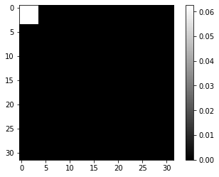
Similarly, we can also rely on a nested for loop to implement a two-dimensional square pulse of duration $N$, defined as

\begin{equation}\sqcap_{L}(m, n) = \begin{cases} &\frac{1}{L^2}, 0 \leq m, n < L, \\ &0, m, n \geq L.\end{cases}\end{equation}

class sq_pulse_2D():
    def __init__(self, N, L):

        self.N=N
        self.L=L
        self.samples=N*N

    def solve(self):
        sq_pulse=np.zeros([self.N, self.N], dtype=np.float)
        for i in range(self.L):
            for j in range(self.L):
                sq_pulse[i,j] = 1/self.L/self.L
            
        return sq_pulse, self.samples

We plot an examples of 2-D square pulse below:

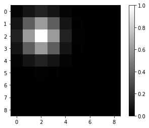
An uncorrelated, two-dimensional Gaussian pulse centered at $\mu$, on the other hand, can be defined as

\begin{equation}\mathbf{G}_\sigma = e^{- [(m – \mu)^2 + (n – \mu)^2]/(2 \sigma^2)}, \end{equation}

and its implementation is shown in the code snippet below.

class Gaussian_2D():
    def __init__(self, N, mu, sigma):
        
        self.N=N
        self.mu=mu
        self.samples=N*N
        self.sigma=sigma

    def solve(self):
        gaussian=np.zeros([self.N, self.N], dtype=np.float)
        for i in range(self.N):
            for j in range(self.N):
                gaussian[i,j] = np.exp(-((i-self.mu)*(i-self.mu)+(j-self.mu)*(j-self.mu))/2/self.sigma/self.sigma)
            
        return gaussian, self.samples

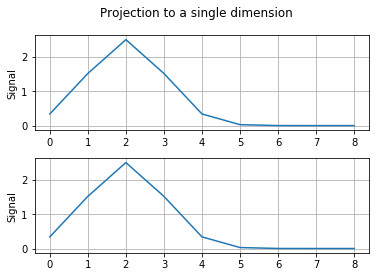
We similarly plot an examples of 2-D Gaussian signal and its projection below:

Two-Dimensional DFT and iDFT

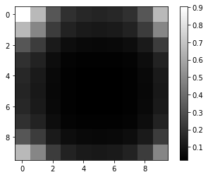
We proceed to consider DFT for two-dimensional signals, which is defined as

\begin{equation}
{\bbX(k,l)} := {\frac{1}{\sqrt{MN}}}\sum_{{m=0}}^{{M-1}} \sum_{{n=0}}^{{N-1}} {\bbx(m,n)}e^{ -j2\pi{k}{m}/M} e^{-j2\pi{l}{n}/N}.
\end{equation}

We can create a class in Python following the above expression, and plot the DFT of a 2-D Gaussian signal with $\mu=0$ and $\sigma=2$ as an example:

Similarly, the iDFT for two-dimensional signals is defined as

\begin{align}
{\tilde{\bbx}(m,n)} &:= \frac{1}{{\sqrt{MN}}} \sum_{{k=0}}^{{M-1}} \sum_{{l=0}}^{{N-1}} {\bbX(k,l)} e^{j 2\pi{k}{m}/M}e^{j 2\pi{l}{n}/N} \nonumber\\ &= \frac{1}{{\sqrt{MN}}} \sum_{{k=-M/2+1 }}^{{M/2}} \sum_{{l=-N/2 +1}}^{{N/2}} {\bbX(k,l)}e^{j 2\pi{k}{m}/M}e^{j 2\pi{l}{n}/N}.
\end{align}

We create a class in Python to run the iDFT, and recover the Gaussian signal from the obtained DFT above:

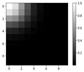
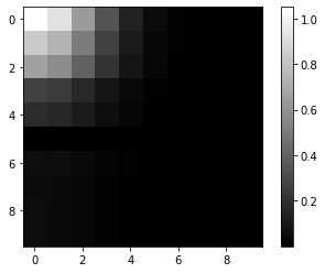
Image De-noise and Filtering

We now de-noise corrupted images by using spatial information about the signal. As introduced in the lab assignment, we could do it by averaging the value of nearby pixels. Recall that averaging is a form of low-pass filtering and thus, we can de-noise 2-D signals by filtering. Specifically, filtering is represented as a convolution with the filter impulse response and in the two-dimensional case, the convolution of two signals $\bbx$ and $\bby$ is defined as

\begin{align}\label{eqn_2d_convolve} [\bbx \ast \bby ] (m,n):&= \sum_{{k=-\infty}}^{{\infty}} \sum_{{l=-\infty}}^{{\infty}} {x(k,l)}{y(m – k,n – l)} \nonumber \\ {}&= \sum_{{k=0}}^{{M-1}} \sum_{{l=0}}^{{N-1}} {x(k,l)}{y(m – k,n – l)} \end{align}

In image processing, it is common to use Gaussian filters for de-noising. In other words, we convolve the image with the Gaussian pulse $\bbG_\sigma$ to obtain

\begin{equation}\label{eqn_denoising} \tbx_{\text{de-noised}} = \bbG_{\sigma} \ast \bbx. \end{equation}

We build a class in Python to do the Gaussian filtering, where we use the function “scipy.signal.convolve2d”. Take the provided imageA as an example, and we plot the denoised below:

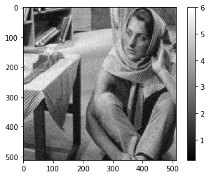
By comparing with the original signal, we observe obvious improvements.

Code Links

The provided code mentioned in the lab assignment can be downloaded from the folder ESE224_Lab8_providedcode.zip. This file contains the provided python classes, but note that the file itself does not perform any computation.

• $\p{discrete\_signal.py}$: This file defines the functions that generate different types 2-D signals and perform the DFT and iDFT.
• $\p{ESE224\_Lab8\_Main.py}$: This file defines the functions that we used to solve the problems in the lab assignment, instantiating objects when necessary. This is also where the plots are created.