
Lab2: Discrete Fourier Transform
We have now seen the DFT expressed as abstract mathematical notation, but how can we implement this in the real world? In this lab, we will code a DFT function in Python, and then use this to explore the DFTs of some signals we have seen in class (square pulse) and some that we have not (triangular pulse, Parzen windows, raised cosine, Gaussian, and Hamming windows). We will then prove some of the important properties of the DFT – conjugate symmetry, energy conservation (Parseval’s Theorem), and linearity, and conservation of inner products (Plancherel’s Theorem).
We will see some more applications of the DFT as it pertains to some real-world signals that we are all familiar with – musical tones. By using the DFT, we will be able to investigate the spectra of an A note and the “Happy Birthday” song that we coded in the last lab. Finally, we will tie all this together to investigate the energy composition of “pure” notes, as well as those that are characterized by harmonics – that is, “real” notes of various instruments.
• Click here to download the assignment.
Spectrum of Pulses
In this first part of the lab we will consider pulses and waves of different shapes to understand what information can be gleaned from spectral analysis. Our goal in this part of the lab is to plot different signals as well as their discrete Fourier transform in order to understand how the signal in time is represented in frequency. Our first example will be a square pulse$\sqcap_M(n)$. According to the definition, the components of this signal are given by, \begin{alignat}{2}\label{eqn_lab_dft_square_pulse} The square pulse is a signal that has a sharp transition, namely, its value changes from the top value to $0$ in just an instant. This sharp transition is expressed in the spectrum by showing a slow decay. This means that even though $90.32
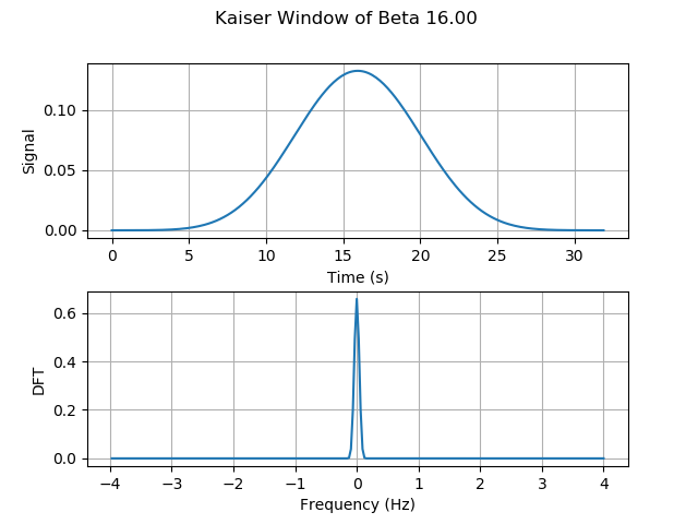
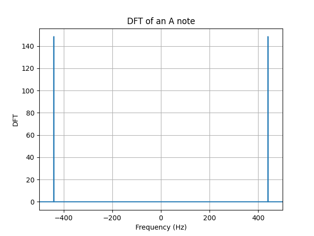
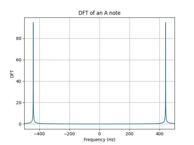
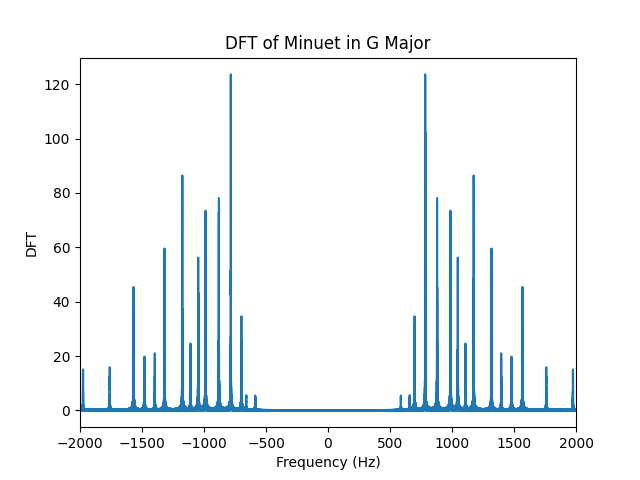
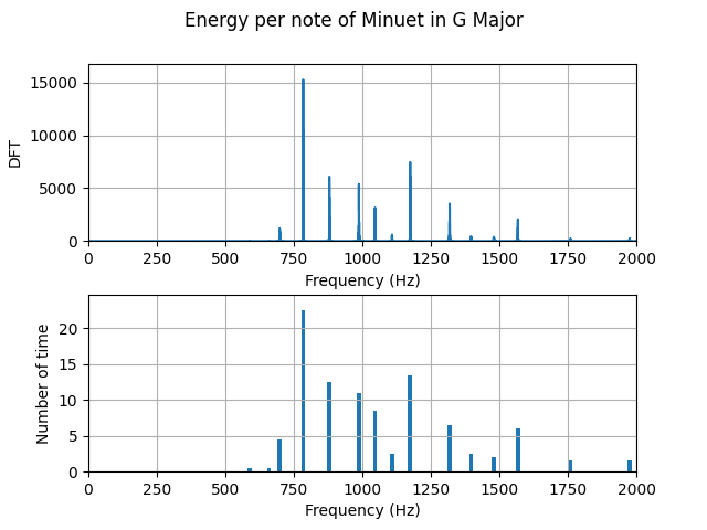
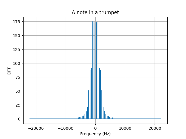
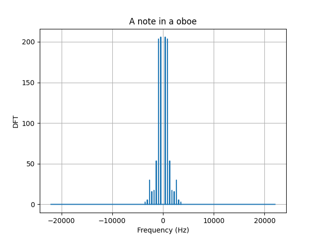
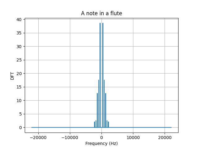
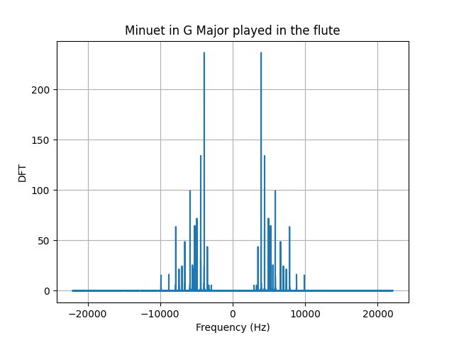
Our second example will be a smoother signal, a signals whose variation is slower. In this case, we will study the triangular pulse $\wedge_M (n)$, this signal goes up and down at a constant rate. According to the definition, the components of this signal are given by, \begin{alignat}{2}\label{eqn_lab_dft_triangular_pulse} The triangular pulse is a smoother signal, thus less components of high frequency need to be added to reconstruct a triangular pulse. This intuition translates into a discrete Fourier transform that shows less components of higher frequencies. In this case, also the $95.71%$ of the energy is contained within the $[-1/4,1/4]$ frequency interval. Recall that this show a $5%$ increment to its square pulse counterpart. Our main takeaway here is, the smoother the signal, the more energy that will be contained within smaller frequencies of the spectrum. The last signal we will work with is the kaiser window, this window was created by Jaimes Kaiser and its applications today are related to the Advanced Audio Coding digital audio format. The equation in this case is not trivial and little intuition can be built upon it. Nevertheless, we can see the signal in time and test the two takeaways we have constructed together. To construct this signals, you can use the class discrete signal. The first property we are asked to show is conjugate symmetry for real signals $x(n)$. This property plays a major role in the way we plot DFTs, you may have noticed that all of the ones we ploted are symmetric around zero. We begin by writing down the definition of the DFT for $X(k)^*$, \begin{align} X^*(k) &= \Bigg(\sum_{n = 0}^{N-1} x(n) e_{kN}^* (n)\Bigg)^* \\ \begin{align} X^*(k) &= \frac{1}{\sqrt{N}}\sum_{n = 0}^{N-1} x(n) exp(- j 2 \pi (-k) n / N)\\ We will next show that the energy conservates, namely that the energy of the signal in time is equal to the energy of the signal in frequency. This theorem is called, Parseval’s Theorem. Letting $X=\ccalF(x)$ be the DFT of signal $x$ and restricting the DFT $X$ to a set of $N$ consecutive frequencies, we are asked to prove that the energies of $x$ and the restricted DFT are the same, \begin{align} Notice that the innermost summation is the inner product between 2 complex exponentials, which is a delta function due to orthonormality. Note here, that the fact that $k$ goes from $N_0$ to $N_0+N-1$ does not affect the fact taht complex exponential are orthogonal. Recall from Lab 1, exercise 1.2, that complex exponentials that are $N$ apart are equivalent. \begin{align} \sum_{k=N_0}^{N_0+N-1}|X(k)|^2&=\sum_{n=0}^{N-1}\sum_{\tilde n=0}^{N-1} x(n) x^*(\tilde n) \left[\frac{1}{N}\sum_{k=N_0}^{N_0+N-1} \langle e_{n N} , e_{\tilde n N} \rangle \right]\\ Since all terms where $\tilde n − n \neq 0$ are equal to zero due to the delta function, we can remove the summation in $\tilde n$ to get \begin{align} \sum_{k=N_0}^{N_0+N-1}|X(k)|^2 &=\sum_{n=0}^{N-1} x(n) x^*(n) \\ &=|| x||^2 The DFT satisfies the linearity property, which means that the DFT of a linear combination of signals is the linear combination of the respective DFTs of the individual signals. This can be formalized as follows, \begin{equation}\label{eqn_lab_dft_properties_linearity} To show it, we write down the definition of DFT for both $\ccalF(x)$ and $\ccalF(y)$ and we operate from there, \begin{align} Essencially, we conclude that the linear combination of internal products is linear, something that was expected. Let $X=\ccalF(x)$ be the DFT of signal $x$ and $Y=\ccalF(y)$ be the DFT of signal $y$. Restrict the DFTs $X$ and $Y$ to a set of $N$ consecutive frequencies. Prove that the inner products $\langle x, y \rangle$ between the signals and $\langle X, Y \rangle$ between the restricted DFTs are the same, \begin{equation}\label{eqn_lab_dft_parseval_2} \begin{align} Notice that we used the fact that the DFT of a signal of length $N$ evaluated at $k$ is equal to the value of the signal at $k+N$. This allows us to shift the sum in the last equality. This is a property that the DFT inherits from the complex exponential and is the basic idea behind the concept of ‘chop and shift’. In this part of the lab we will study the spectrum of different tones, songs and harmonics. To begin with, let’s study the DFT of an A note. To generate an A note, we will sample a cosine of frequency $f_0 = 440Hz$ at a sampling frequency of $f_s=44100$ for $T=2s$. The following plot, shows the desired DFT. We can also conclude that Parseval’s Theorem holds as the energy of the signal computed in the time domain and in the frequency domain are both $44100 J$. We know that the whole signal is contained within $\pm f_0$ as we are sampling a cosine signal. An interesing effect called $leakage$ occurs when the signal is sampled for a time that is not a multiple of its period $T_0$. In order not to see perfect deltas, and visualize the spectral leakage effect we should change T to a number that is not a multiple of 1/f_0. Spectral leakage is a result of time T that leads to an uneven number of oscillations. Try for instance setting T=880.5/f_0. You will see the DFT widening out near the bottom of the spikes. To make things more interesting, we can work with a song. Arguably, one of the most beautiful songs ever composed is Minuet in G Major, a minimalistic interpretation of this song can be found here. If we plot the DFT of this art piece, we will encounter several delta, each corresponding to a different frequency value, which we now know, corresponds to a different note. We can cross check that the energy of each note is indeed correlated with the time each note is played. This may have seem magical a couples of weeks ago, but now you are able to see the relationship between signals and their spectrum. Besides, we can even make the spectrum confess what the ear can’t distinguish. However, musical intruments generate rich sounds not just simple notes. To be able to simulate this, we will need to add $harmonics$ of the $fundamental$ frequency. The weight each harmonic has is unique per instrument and allow musicians to create beautiful pieces like the one we mentioned before. We can try to simulate to the sound of at least a couple of instruments by assigning weigths to their harmonics as follows. In both the oboe and the flute, $90%$ of the energy is contained within the first two harmonics. In the trumpet and clarinet thought, we need $4$ and $6$ harmonics respectively to reach $90%$ of the total energy. We can conclude that these two last instruments generate a more plain sound in frequency. By ploting the song in the flute we see a richer spectrum, namely more frequencies come into play when the same song is played. This richer spectrum is what makes songs sound more harmonic. Now you can also claim that you know what this really means! The code described here can be downloaded from the folder ESE224_Lab2.zip. This folder contains the following 4 files:
&\sqcap_M(n) = \frac{1}{\sqrt{M}} && \qquad \text{if } 0\leq n < M, \nonumber\ \\
&\sqcap_M(n) = 0 && \qquad \text{if } n \geq M.
\end{alignat}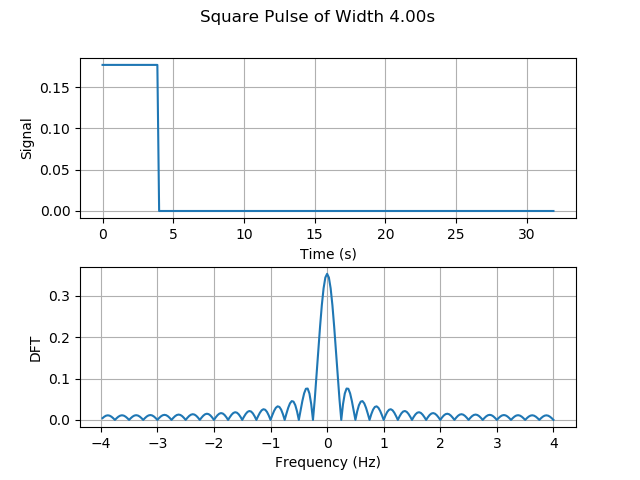
&\wedge_M(n) = n && \qquad \text{if } 0 \leq n < M/2, \nonumber\ \\
&\wedge_M(n) = (M – 1) – n && \qquad \text{if } M/2 \leq n < M, \nonumber\ \\
&\wedge_M(n) = 0 && \qquad \text{if } n \geq M.
\end{alignat}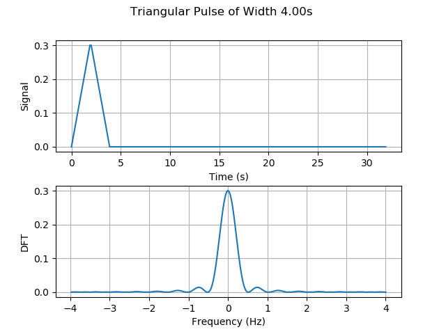
Properties of the DFT
Conjugate symmetry
&= \frac{1}{\sqrt{N}}\Bigg(\sum_{n = 0}^{N-1} x(n) exp(-j 2 \pi k n / N)\Bigg)^*\\ &= \frac{1}{\sqrt{N}}\sum_{n = 0}^{N-1} x(n) \Bigg(exp(- j 2 \pi k n / N)\Bigg)^*
\end{align}
The last equality holds since the conjugate of the sum is the sum of the conjugates, and $x(n)$ is a real signal, so $x(n)^*=x(n)$. We finally obtain,
&= X(-k)
\end{align}Energy conservation (Parseval’s Theorem)
\begin{equation}\label{eqn_lab_dft_parseval}
\sum_{n=0}^{N-1} |x(n)|^2 = {|x|^2 = |X|^2}
= \sum_{k=N_0}^{N_0+N-1} |X(k)|^2.
\end{equation}
The constant $N_0$ in \eqref{eqn_lab_dft_parseval} is arbitrary. The energy of each individual term of the DFT can be obtained as,
|X(k)|^2&= X(k) X^* (k) &= \left[\frac{1}{\sqrt{N}} \sum_{n=0}^{N-1}x(n) e^{- j 2 \pi k n /N } \right]\left[\frac{1}{\sqrt{N}}\sum_{\tilde n=0}^{N-1}x(\tilde n)^* e^{ j 2 \pi k \tilde n /N} \right]
\end{align}
Now, we can take the summation of the $N$ consecutive terms starting at $N_0$,
\begin{align}
\sum_{k=N_0}^{N_0+N-1}|X(k)|^2&=\sum_{k=N_0}^{N_0+N-1} X(k) X^*(k)\\ &=\sum_{k=N_0}^{N_0+N-1} \left[\frac{1}{\sqrt{N}}\sum_{n=0}^{N-1}x(n) e^{- j 2 \pi k n /N } \right]\left[\frac{1}{\sqrt{N}}\sum_{\tilde n=0}^{N-1}x(n)^* e^{ j 2 \pi k \tilde n /N } \right]
\end{align}
We can simplify this complicated summation by changing the order to sum over $k$ first
instead of $n$ and $\tilde n$. In doing so, we can also pull $x(n)$ and $x(\tilde n)$ out of the inner summation since they don’t depend on $k$,
\begin{align}
\sum_{k=N_0}^{N_0+N-1}|X(k)|^2&=\sum_{n=0}^{N-1}\sum_{\tilde n=0}^{N-1} x(n) x^*(\tilde n) \left[\frac{1}{N}\sum_{k=N_0}^{N_0+N-1} e^{- j 2 \pi k n /N } e^{ j 2 \pi k \tilde n /N } \right] \end{align}
&=\sum_{n=0}^{N-1}\sum_{\tilde n=0}^{N-1} x(n) x^*(\tilde n) \delta(\tilde n – n) \end{align}
\end{align}
Finishing the proof.Linearity
\ccalF(ax + by) = a\ccalF(x) + b \ccalF(y).
\end{equation}
\ccalF(ax + by)(k) &= \frac{1}{\sqrt{N}}\sum_{n=0}^{N-1} (ax(n)+by(n))e^{-j2\pi kn /N}\\
&= \frac{1}{\sqrt{N}}\sum_{n=0}^{N-1} ax(n)e^{-j2\pi kn /N}+by(n)e^{-j2\pi kn /N}\\
&= \frac{1}{\sqrt{N}}\sum_{n=0}^{N-1} ax(n)e^{-j2\pi kn /N}+\frac{1}{\sqrt{N}}\sum_{n=0}^{N-1}by(n)e^{-j2\pi kn /N}\\
&= a\frac{1}{\sqrt{N}}\sum_{n=0}^{N-1} x(n)e^{-j2\pi kn /N}+b\frac{1}{\sqrt{N}}\sum_{n=0}^{N-1}by(n)e^{-j2\pi kn /N}\\
&= a\ccalF(x) + b \ccalF(y).
\end{align}Conservation of inner products (Plancherel’s Theorem)
\sum_{n=0}^{N-1} x(n)y^*(n) = \langle x, y \rangle = \langle X, Y \rangle = \sum_{k=N_0}^{N_0+N-1} X(k)Y^*(k)
\end{equation}
The constant $N_0$ in \eqref{eqn_lab_dft_parseval_2} is arbitrary. Observe that the result in part Energy conservation (Parseval’s Theorem) is a particular case of Plancherel’s Theorem. This statement may sound complicated, but the proof is far from it. Starting with the definition, we can show that.
\sum_{n=0}^{N-1}\langle x(n),y(n)\rangle&=\sum_{n=0}^{N-1} x(n)y(n)^*\\ &=\sum_{n=0}^{N-1} x(n) \Bigg (\frac{1}{\sqrt{N}} \sum_{k=0}^{N-1} Y(k) e^{2\pi j n /N } \Bigg )^*\\
&=\sum_{n=0}^{N-1} x(n) \Bigg (\frac{1}{\sqrt{N}} \sum_{k=0}^{N-1} Y(k)^* e^{-2\pi j n /N } \Bigg )\\
&=\sum_{k=0}^{N-1} Y(k)^* \Bigg (\frac{1}{\sqrt{N}} \sum_{n=0}^{N-1} x(n) e^{-2\pi j n /N } \Bigg )\\
&=\sum_{k=0}^{N-1} Y(k)^* X(k)\\
&=\sum_{k=N_0}^{N+N-1} Y(k)^* X(k)
\end{align}Spectra of musical tones
Code Links