Lab1: Discrete Complex Exponentials

Where shall we begin? From the very beginning. And in the beginning there was nothing. But then there was time. Our exploration of information processing starts from an exploration of the notion of time. More precisely, from the notion of rate of change. This is because different rates of change are often associated with different types of information. In a picture of a face, no change means you are looking at hair, foreheads, or cheeks. Rapid change means you are looking at a hairline, a pair of eyes, or a pair of lips. Different vowels are associated to different frequencies. So are musical tones. The lull of the ocean spreads across all frequencies. Weather changes occur over days. Season changes over months. Climate changes over years.

The Fourier transform is the mathematical tool that uncovers the relationship between different rates of change and different types of information. In order to define Fourier transforms, which we will do in Lab 2, we first have to study discrete complex exponentials and some of their properties. This is the objective of this Lab.

• Click here to download the assignment.

In this first part of the lab, we are asked to generate and display some discrete complex exponentials. This is a little bit of busy work that we are undertaking so that we can use the code to explore some properties of these signal. Like the fact that some of them are equivalent to each other, that some other ones are conjugates of each other, and that they form an orthonormal basis of the space of signals of a given duration

import numpy as np
import matplotlib.pyplot as plt
import math
import cmath

class ComplexExp(object):
   def __init__(self, k, N):
        self.k = k
        self.N = N

        self.n = np.arange(N)

        # Vector containing elements of the complex exponential
        self.exp_kN = np.exp(2j*cmath.pi*self.k*self.n / self.N)
        self.exp_kN *= 1 / (np.sqrt(N))

        # Real and imaginary parts
        self.exp_kN_real = self.exp_kN.real
        self.exp_kN_imag = self.exp_kN.imag

# Importing the class we just created
from cpx_exp import ComplexExp

def q_11(N, k_list):

    for k in k_list:
        # Creates complex exponential object with frequency k and duration N
        exp_k = ComplexExp(k, N)
        # Real and imaginary parts
        cpx_cos = exp_k.exp_kN_real
        cpx_sin = exp_k.exp_kN_imag
        # Plots real and imaginary parts
        cpx_plt = plt.figure()
        plt.stem(exp_k.n, cpx_cos, 'tab:blue', markerfmt='bo')
        plt.stem(exp_k.n, cpx_sin, 'tab:green', markerfmt='go')

if __name__ == '__main__':
    list_of_ks = [0, 2, 9, 16]
    duration_of_signal = 32
    q_11(duration_of_signal, list_of_ks)

Since we need to repeat the procedure for different frequencies, the function $\p{q\_11}$ above takes as argument a list of frequencies and iterates over the frequencies in the list. Note that you can also create a function that takes only one frequency at a time, and run it multiple times. To plot the imaginary and real pars of the discrete complex exponential, we can use the $\p{stem}$ function from matplotlib. To save the plots locally, you can use the $\p{savefig}$ method.

Once we have defined the $\p{ComplexExp}$ class, we can use it to solve problems 1.2 – 1.4 — all we need to do is to create new objects with the particular discrete frequencies we need. In part 1.2, for example, we need to generate complex exponentials of the same duration and frequencies $k$ and $l$ that are $N$ apart. Running the code snippet above with $N = 32$, $k=3$ and $l = 35$, for example, we obtain Figures 1 and 2. Note that — as expected from the definition of a discrete complex exponential in \eqref{eq:disc_cpx_exp} — the two signals are identical.

Figure 1: $k$ = 3

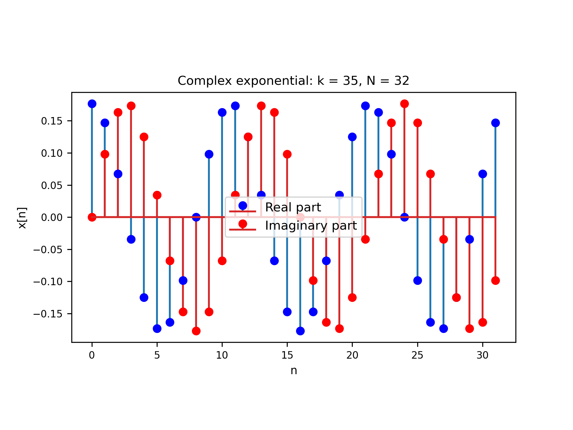
Figure 2: $k$ = 35

Similarly, we can use the same code snippet to solve part 1.3, where we now want to evaluate the behavior of discrete complex exponentials of same duration but opposite frequencies. Let us then take $N=32$, $k = \pm 3$, and rerun the code with these values to create Figures 3 and 4. Note that the two discrete complex exponentials below have the same real part, but opposite imaginary parts, that is, the signals are conjugate of each other. To see why that happens, note that we can take

\begin{equation} \begin{aligned} \text{Re} \left( e_{-kN} (n) \right) &= \frac{1}{\sqrt{N}} \cos (-2\pi k n / N) = \frac{1}{\sqrt{N}} \cos (2\pi k n / N) = \text{Re} \left( e_{kN} (n) \right) , \\ \text{Im} \left( e_{-kN} (n) \right) &= \frac{1}{\sqrt{N}} \sin (- 2\pi k n / N) = – \frac{1}{\sqrt{N}} \sin (2\pi k n / N) = – \text{Im} \left( e_{kN} (n) \right). \end{aligned} \end{equation}

Figure 3: $k$ = 3

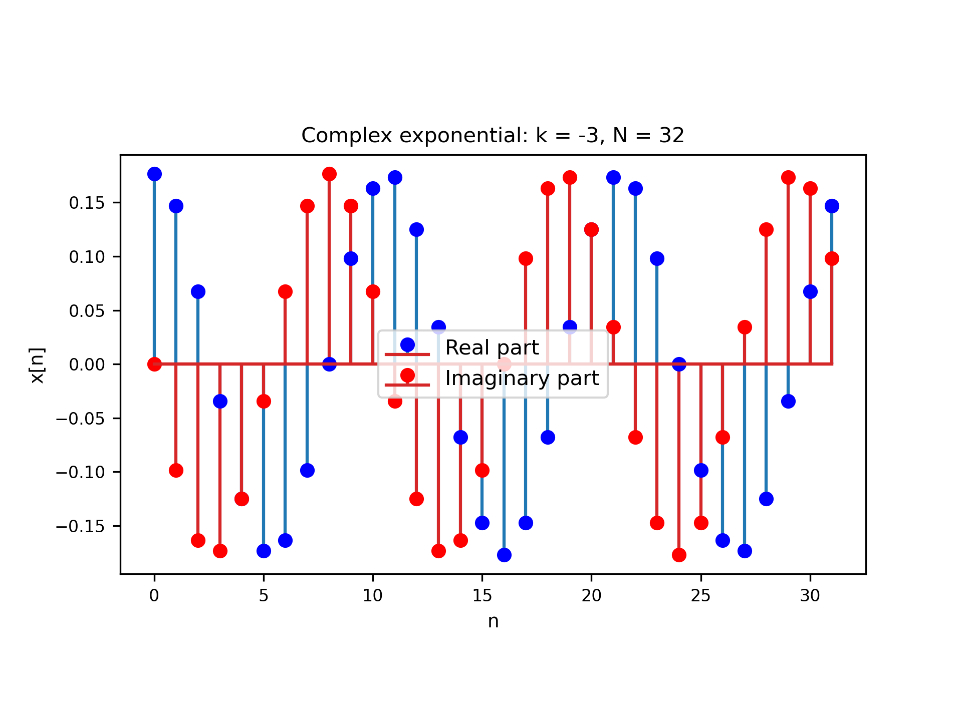
Figure 4: $k$ = -3

In part 1.5, on the other hand, we are asked to do something slightly different: here, we need to implement a function that computes the inner product $\langle e_{kN}, e_{lN}\rangle$ between all pairs of discrete complex exponentials of length $N$ and discrete frequencies $k, l = 0, \dots, N-1$. For two signals $x$ and $y$ of duration $N$, the inner product is defined as

\begin{equation} \langle x,y \rangle := \sum_{n = 0}^{N-1} x(n)y^*(n). \end{equation}

Note that, if we take the signals as column vectors, then we can simply compute the inner product as

\begin{equation} \langle x,y \rangle := y^H x, \end{equation}

with $y^H$ standing for the Hermitian transpose of $y$. That’s how the code snippet below computes the inner products.

def q_15(N):
    k_list = np.arange(N)
    l_list = np.arange(N)

    cpx_exps = np.zeros((N,N), dtype=np.complex)
    for k in k_list:
        cpx_exp = ComplexExp(k, N)
        cpx_exps[:, k] = cpx_exp.exp_kN

    cpx_exps_conj = np.conjugate(cpx_exps)

    # Option 1: computing inner products simultaneously
    res = np.round(np.matmul(cpx_exps_conj, cpx_exps).real)
    print ("\n Matrix of inner products: Mp =")
    ls.print_matrix(res)
        
    # Option 2: using for loops
    opt2 = np.zeros((N,N), dtype=np.complex)
    for k in k_list:
        for l in l_list:
            r = np.dot(cpx_exps_conj[:, k], cpx_exps[:, l])
            opt2[k, l] = r
            opt2[l, k] = r
    
    res2 = opt2.real 
    print ("\n Matrix of inner products: Mp = ")
    ls.print_matrix(res2)

    return res

Since we are computing $N \times N$ inner products, we store the resulting inner products in an $N \times N$ matrix. Here we show two options to compute that matrix. Option 2 simply loops over all the discrete frequencies $k, l = 0, \dots, N-1$. Option 1, on the other hand, constructs a matrix made up by column vectors representing the $N$ complex exponentials, and then computes the inner products simultaneously. Note that the two solutions are equivalent! To see the resulting matrix, we can use, for example, the $\p{print\_matrix}$ function from that first post on object oriented programming in Python. Or use the matplotlib package to display the resulting matrix. Either way, the key observation here is that discrete complex exponentials have unit energy and are orthogonal to each other; and thus, they form an orthonormal set. That is one of the reasons why we can use a set of discrete complex exponentials to represent discrete signals in the frequency domain, as we will see in the next few weeks.

Analyzing Complex Exponentials

In Part 1, we used some numerical experiments to illustrate two very important properties of discrete complex exponentials: orthogonality and equivalence. Let us now study these properties analytically.

First we prove that two discrete complex exponentials $e_{kN}(n)$ and $e_{lN}(n)$ of same duration $N$ and discrete frequencies $k, l$ such that $k – l = N$ are equivalent, that is, $e_{kN}(n) = e_{lN}(n)$ for all times $n = 0, \dots, N – 1$:

\begin{equation} \frac{e_{kN} (n)}{e_{lN} (n)} = \frac{\frac{1}{\sqrt{N}} \, e^{j2\pi k n /N}}{\frac{1}{\sqrt{N}} \, e^{j2\pi ln /N}} = e^{j2\pi{(k – l)}{n}/N} = e^{j2\pi n} = 1.\end{equation}

Note that the same holds whenever the difference between $k$ and $l$ is a multiple of $N$, that is, $k – l = \alpha N$ for some $\alpha \in \mathbb{Z}:$

\begin{equation} \frac{e_{kN} (n)}{e_{lN} (n)} = \frac{\frac{1}{\sqrt{N}} \, e^{j2\pi k n /N}}{\frac{1}{\sqrt{N}} \, e^{j2\pi ln /N}} = e^{j2\pi{(k – l)}{n}/N} = e^{j2\pi \alpha n} = 1.\end{equation}

Now, we will prove that two complex exponentials that are not equivalent — that is, the difference between $k$ and $l$ is not a multiple of $N$ —are orthogonal to each other.

First, recall that the inner product of two signals $x$ and $y$ of duration $N$ is given by

\begin{equation} \langle x,y \rangle := \sum_{n = 0}^{N-1} x(n)y^*(n). \end{equation}

Using the formula above to compute the inner product between two (non-equivalent) complex exponentials $e_{kN}(n)$ and $e_{lN}(n)$, we get

\begin{equation}
\begin{aligned}
\langle e_{kN}(n), e_{lN}(n) \rangle &= \sum_{n = 0}^{N-1} e_{kN}(n)e_{lN}^*(n) = \frac{1}{N} \sum_{n = 0}^{N-1} e^{j2\pi k n /N} e^{-j2\pi ln /N} \\ &= \frac{1}{N} \sum_{n = 0}^{N-1} e^{j2\pi (k – l) n /N} = \frac{1}{N} \sum_{n = 0}^{N-1} \left[ e^{j2\pi (k – l) /N} \right]^n .
\end{aligned}
\end{equation}

Note that the above expression is the sum of a finite, geometric series. Using the formula for a finite geometric sum, we then have

\begin{equation} \sum_{n = 0}^{N-1} e_{kN}(n)e_{lN}^*(n) = \frac{1}{N} \frac{1 – \left[ e^{j2\pi (k – l) /N} \right]^{N – 1 + 1}}{1 – e^{j2\pi (k – l) /N}} = \frac{1}{N} \frac{1 – e^{j2\pi (k – l)} }{1 – e^{j2\pi (k – l) /N}} \end{equation}

But $e^{j2\pi (k – l)} = \left[ e^{j 2 \pi}\right]^{(k – l)} = 1$ and thus

\begin{equation} \sum_{n = 0}^{N-1} e_{kN}(n)e_{lN}^*(n) = 0. \end{equation}

This shows that non-equivalent discrete complex exponentials are orthogonal. Now, if we compute the energy of a discrete complex exponential, we get

\begin{equation}
\begin{aligned} \| e_{kN}(n) \|^2 &= \langle e_{kN}(n), e_{kN}(n) \rangle \\ &= \sum_{n = 0}^{N-1} e_{kN}(n)e_{kN}^*(n) = \frac{1}{N} \sum_{n = 0}^{N-1} e^{j2\pi (k – k) n /N} = \frac{1}{N} \sum_{n = 0}^{N-1} 1 = 1.
\end{aligned}
\end{equation}

Thus, discrete complex exponentials have unit norm. Since non-equivalent complex exponentials are orthogonal, we conclude that a collection of $N$ consecutive discrete complex exponentials form an orthonormal set. Note that we can redo the analysis above for shifted complex exponentials and still get the same conclusions: if the difference between $k$ and $l$ is a multiple of $N$, then the discrete complex exponentials will be equivalent. If the difference between $k$ and $l$ is not a multiple of $N$, however, then the discrete complex exponentials will be orthogonal — that holds because the phase shifts cancel each other out. Similarly, allowing for $k$ and $l$ to be real will not change our conclusions: the discrete complex exponentials will be equivalent if $k – l$ is a multiple of $N$ and orthogonal otherwise.

Generating and Playing Musical Tones

In this section, we explore the use of discrete signals as representations of continuous signals that exist in the real world. We start with the implementation of a function that, given the sampling frequency $f_s$, the duration $T$ of the continuous signal, and the frequency $f_0$ of a continuous cosine, returns a discrete cosine $x(n)$ given by

\begin{equation}
x(n) = \cos (2 \pi (f_0 / f_s) n ) = \cos (2 \pi f_0 nT_s )
\label{eq:disc_cos_sampled}
\end{equation}

Since a discrete cosine corresponds to the real part of a discrete complex exponential, we can use our implementation of a discrete complex exponential to solve this problem. First, note that we have the duration of the continuous signal, $T$, and the sampling $f_s$, and thus we can compute the number of samples or the duration of the discrete signal, $N$,

\begin{equation}
N = Tf_s
\end{equation}

When $T$ is not a multiple of $T_s$, we can reduce it to the largest multiple of $T_s$ smaller than $T$, which can be achieved with the function $\p{floor}$ from the math package.

def cexpt(f, T, fs):

    N = math.floor(T * fs)
    k = N * f / fs
    # Complex exponential
    cpx_exp = ComplexExp(k, N)
    x = cpx_exp.exp_kN
    x = np.sqrt(N) * x

    return x, N

def q_31(f, T, fs):
    cpxexp, num_samples = cexpt(f, T, fs)
    cpxcos = cpxexp.real

To compute the discrete frequency, we use the relation

\begin{equation} k = N \frac{f_0}{f_s}.\end{equation}

Once we have that discrete frequency, we can then create a discrete complex exponential with frequency $k$ and duration $N = T f_s$. As a discrete complex exponential is normalized, we multiply it by $\sqrt{N}$ to retrieve equation \eqref{eq:disc_cos_sampled}. Finally, recall that the cosine is the real part of a complex exponential — so we can retrieve the discrete cosine by using $\p{cpxexp.real}$.

We can use the same idea to play musical notes. The $A$ note, for example, corresponds to an oscillation at the frequency $f = 440 Hz$. But we just implemented a function that, given the sampling frequency $f_s$, the frequency of the continuous oscillation $f_0$, and the duration of the continuous signal, $T$, returns the associated discrete cosine. Hence, we can simply do:

from scipy.io.wavfile import write

def q_32(f0, T, fs):
    cpxexp, num_samples = cexpt(f0, T, fs)
    Anote = cpxexp.real
    write("Anote.wav", fs, Anote.astype(np.float32))

if __name__ == '__main__':
    f0 = 440
    T = 2
    fs = 44100
    q_32(f0, T, fs)

To play the musical tone, we import the $\p{write}$ function from the scipy library to write a numpy array as an .wav file — that we can then open with any media player.

To play other musical tones — and to use the piano key number instead of the frequency $f_i$ as an argument, we can modify the function accordingly: <\p>

def q_33(note, T, fs):

    fi = 2**((note - 49) / 12)*440
    cpxexp, num_samples = cexpt(fi, T, fs)
    q33note = cpxexp.real
    write("q33note.wav", fs, q33note.astype(np.float32))

And if we want to play a song, all we need to do is play the notes in the right order. Then we can, for example, create a list with all the notes in our song, find the corresponding discrete cosines, and create a single array with the entire song.<\p>

def q_34(list_notes, list_times, fs):
    song = []
    for note, note_time in zip(list_notes, list_times):
        fi = 2**((note - 49) / 12)*440
        x, N = cexpt(fi, note_time, fs)
        song = np.append(song, x.real)
        song = np.append(song, np.zeros(10))

    write("q34_song.wav", fs, song.astype(np.float32))

Code links

The code described here can be downloaded from the folder ESE224_Lab1.zip. This folder contains the following two files:

$\p{cpx\_exp.py}$: The class $\p{ComplexExp}$ is defined in this file — but note that the file itself does not perform any computation.

$\p{ESE224\_Lab1\_Main.py}$: This file defines the functions that we used to solve the problems in the lab assignment, instantiating objects of the class $\p{ComplexExp}$ when necessary. This is also where the plots and the audio files are created.